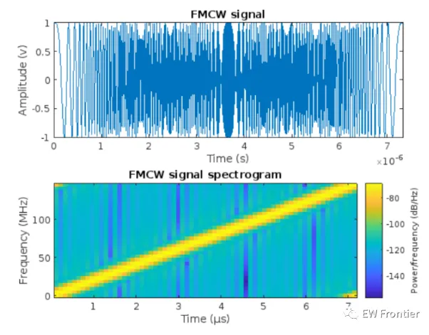
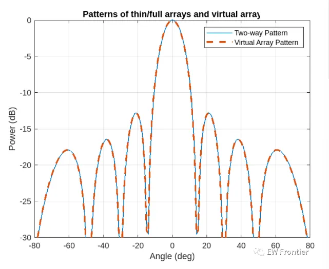
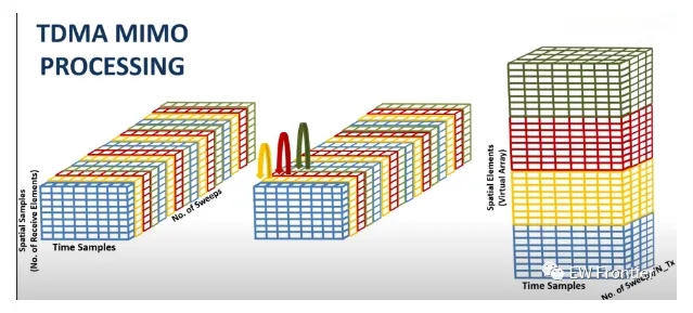
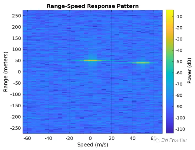
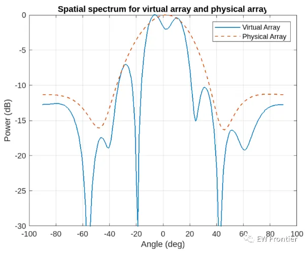
.rtcContent { padding: 30px; } .lineNode {font-size: 16pt; font-family: Menlo, Monaco, Consolas, "Courier New", monospace; font-style: normal; font-weight: normal; }%TDM MIMO Radar signal processing chain basicsfc = 77e9; %typical center freq for automotive radarsc = 3e8;lambda = c/fc;Nt = 2; %no of trasnmittersNr = 4; %no of recievers%defining array characteristicsdt = Nr*lambda/2; %thin array spacingdr = lambda/2; %full array spacingtxarray = phased.ULA(Nt,dt);rxarray = phased.ULA(Nr,dr);ang = -90:90; %field of view (FOV)pattx = pattern(txarray,fc,ang,0,'Type','powerdb');patrx = pattern(rxarray,fc,ang,0,'Type','powerdb');pat2way = pattx+patrx;%Demonstrating the equivalence of the two-way pattern this system %with a virual array of Nt * Nr elements varray = phased.ULA(Nt*Nr,dr);patv = pattern(varray,fc,ang,0,'Type','powerdb');figure(1)helperPlotMultipledBPattern(ang,[pat2way patv],[-30 0],... {'Two-way Pattern','Virtual Array Pattern'},... 'Patterns of thin/full arrays and virtual array',... {'-','--'},[1 2]);%TDM-MIMO Radar Simulation%Defining Waveformwaveform = helperDesignFMCWWaveform(c,lambda);fs = waveform.SampleRate;tm = waveform.SweepTime;sig = waveform();figure(2)subplot(211); plot(0:1/fs:tm-1/fs,real(sig));xlabel('Time (s)'); ylabel('Amplitude (v)');title('FMCW signal'); axis tight;subplot(212); spectrogram(sig,32,16,32,fs,'yaxis');title('FMCW signal spectrogram');%Radar System Setup%only main components are modeled and the effects from other components%are omitted, such as coupler and mixer. % In addition, the antenna is assumed to be isotropic.transmitter = phased.Transmitter('PeakPower',0.001,'Gain',36);receiver = phased.ReceiverPreamp('Gain',40,'NoiseFigure',4.5,'SampleRate',fs);txradiator = phased.Radiator('Sensor',txarray,'OperatingFrequency',fc,... 'PropagationSpeed',c,'WeightsInputPort',true);rxcollector = phased.Collector('Sensor',rxarray,'OperatingFrequency',fc,... 'PropagationSpeed',c);%The Radar has two cars in the FOV with a separation of 20 degrees%Define position and motion of the ego vehicle and the two cars in the FOVradar_speed = 100*1000/3600; % Ego vehicle speed 100 km/hradarmotion = phased.Platform('InitialPosition',[0;0;0.5],'Velocity',[radar_speed;0;0]);car_dist = [40 50]; % Distance between sensor and cars (meters)car_speed = [-80 96]*1000/3600; % km/h -> m/scar_az = [-10 10];car_rcs = [20 40];car_pos = [car_dist.*cosd(car_az);car_dist.*sind(car_az);0.5 0.5];cars = phased.RadarTarget('MeanRCS',car_rcs,'PropagationSpeed',c,'OperatingFrequency',fc);carmotion = phased.Platform('InitialPosition',car_pos,'Velocity',[car_speed;0 0;0 0]);%Channel model is assumed to be free space.channel = phased.FreeSpace('PropagationSpeed',c,... 'OperatingFrequency',fc,'SampleRate',fs,'TwoWayPropagation',true);%Generating the radar data cube recieved by the radarrng(2017);Nsweep = 64;Dn = 2; % Decimation factorfs = fs/Dn;xr = complex(zeros(fs*waveform.SweepTime,Nr,Nsweep));w0 = [0;1]; % weights to enable/disable radiating elementsfor m = 1:Nsweep % Update radar and target positions [radar_pos,radar_vel] = radarmotion(waveform.SweepTime); [tgt_pos,tgt_vel] = carmotion(waveform.SweepTime); [~,tgt_ang] = rangeangle(tgt_pos,radar_pos); % Transmit FMCW waveform txsig = transmitter(sig); % Toggle transmit element w0 = 1-w0; txsig = txradiator(txsig,tgt_ang,w0); % Propagate the signal and reflect off the target txsig = channel(txsig,radar_pos,tgt_pos,radar_vel,tgt_vel); txsig = cars(txsig); % Dechirp the received radar return rxsig = rxcollector(txsig,tgt_ang); rxsig = receiver(rxsig); dechirpsig = dechirp(rxsig,sig); % Decimate the return to reduce computation requirements for n = size(xr,2):-1:1 xr(:,n,m) = decimate(dechirpsig(:,n),Dn,'FIR'); endend%converting the radar data cube generated from the physical array%to the one formed using the virtual arrayxr1 = xr(:,:,1:2:end); %cube recieved by first transmit antennaxr2 = xr(:,:,2:2:end); %cube recieved by first transmit antennaxrv = cat(2,xr1,xr2); %virtual radar data cube%performing range-Doppler processing on the virtual data cube.nfft_r = 2^nextpow2(size(xrv,1));nfft_d = 2^nextpow2(size(xrv,3));rngdop = phased.RangeDopplerResponse('PropagationSpeed',c,... 'DopplerOutput','Speed','OperatingFrequency',fc,'SampleRate',fs,... 'RangeMethod','FFT','PRFSource','Property',... 'RangeWindow','Hann','PRF',1/(Nt*waveform.SweepTime),... 'SweepSlope',waveform.SweepBandwidth/waveform.SweepTime,... 'RangeFFTLengthSource','Property','RangeFFTLength',nfft_r,... 'DopplerFFTLengthSource','Property','DopplerFFTLength',nfft_d,... 'DopplerWindow','Hann');[resp,r,sp] = rngdop(xrv);%the range-Doppler map for the first element in the virtual arrayfigure(3)plotResponse(rngdop,squeeze(xrv(:,1,:)));%performing detection using a manual threshold deduced from%the range-doppler maprespmap = squeeze(mag2db(abs(resp(:,1,:))));ridx = helperRDDetection(respmap,-10);%extracting range cuts of targets for further spatial processingxv = squeeze(sum(resp(ridx,:,:),1))';doa = phased.BeamscanEstimator('SensorArray',varray,'PropagationSpeed',c,... 'OperatingFrequency',fc,'DOAOutputPort',true,'NumSignals',2,'ScanAngles',ang);[Pdoav,target_az_est] = doa(xv);fprintf('target_az_est = [%s]\n',num2str(target_az_est));%demonstrating angular resolution improvment achieved by virtual arraydoarx = phased.BeamscanEstimator('SensorArray',rxarray,'PropagationSpeed',c,... 'OperatingFrequency',fc,'DOAOutputPort',true,'ScanAngles',ang);Pdoarx = doarx(xr);figure(4)helperPlotMultipledBPattern(ang,mag2db(abs([Pdoav Pdoarx])),[-30 0],... {'Virtual Array','Physical Array'},... 'Spatial spectrum for virtual array and physical array',{'-','--'});